Starting With Data
Working With Pandas DataFrames in Python
Learning Objectives
- Explain what a library is, and what libraries are used for.
- Load a Python/pandas library.
- Read tabular data from a file into Python using Pandas using
read_csv. - Learn about the Pandas DataFrame object.
- Learn about data slicing and indexing.
- Perform mathematical operations on numeric data.
- Create simple plots of data.
About Libraries
A library in Python contains a set of tools (called functions) that perform tasks on our data. Importing a library is like getting a piece of lab equipment out of a storage locker and setting it up on the bench for use in a project. Once a library is set up, it can be used or called to perform many tasks.
Pandas in Python
One of the best options for working with tabular data in python is to use the Python Data Analysis Library (a.k.a. pandas). The Pandas library provides data structures, produces high quality plots with matplotlib and integrates nicely with other libraries that use NumPy (which is another Python library) arrays.
Python doesn't load all of the libraries available to it by default. We have to
add an import statement to our code in order to use library functions. To import
a library, we use the syntax import libraryName. If we want to give the
library a nickname to shorten the command, we can add as nickNameHere. An
example of importing the pandas library using the common nickname pd is below.
import pandas as pd
Each time we call a function that's in a library, we use the syntax
LibraryName.FunctionName. Adding the library name with a . before the
function name tells python where to find the function. In the example above, we
have imported pandas as pd. This means we don't have to type out pandas each
time we call a pandas function.
Lesson Overview
We are studying the species and weight of animals caught in plots in a study
area. The data sets are stored in .csv (comma separated value) format. Within
the .csv files, each row holds information for a single animal, and the
columns represent: record_id, month, day, year, plot, species, sex, wgt.
The first few rows of our first file look like this:
"record_id","month","day","year", "plot","species","sex","wgt"

"63","8","19","1977","3","DM","M","40"

"64","8","19","1977","7","DM","M","48"

"65","8","19","1977","4","DM","F","29"

"66","8","19","1977","4","DM","F","46"

"67","8","19","1977","7","DM","M","36"
We want to:
- Load that data into memory in Python.
- Calculate the average weight of all individuals sampled, by species.
- Plot the average weights by species and perhaps by plot too.
We can automate the process above using Python. It's efficient to spend time building the code to perform these tasks because once it's built, we can use it over and over on different datasets that use a similar format. This makes our methods easily reproducible. We can also easily share our code with colleagues and they can replicate the same analysis.
Reading Data Using Pandas CSV
We will begin by locating and reading our survey data which are in CSV format.
We can use Pandas read_csv function to pull the file directly into a
DataFrame.
So What's a DataFrame?
A DataFrame is a 2-dimensional data structure that can store data of different
types (including characters, integers, floating point values, factors and more)
in columns. It is similar to spreadsheets or SQL tables or the data.frame in
R.
First, let's make sure the python Pandas library is loaded. We will import
Pandas using the nickname pd.
import pandas as pd
Let's also import the OS Library. This library allows us to make sure we are in the correct working directory. If you are working in IPython Notebook, be sure to start the notebook in the workshop repository. If you didn't do that you can always set the working directory using the code below.
import os
os.getcwd()
# if this directory isn't right, use the command below to set the working directory
os.chdir("YOURPathHere")
# note the pd.read_csv is used because we imported pandas as pd
pd.read_csv("data/surveys.csv")
The above command yields the output below:
       record_id  month  day  year  plot species  sex  wgt
0              1      7   16  1977     2     NaN    M  NaN
1              2      7   16  1977     3     NaN    M  NaN
2              3      7   16  1977     2      DM    F  NaN
3              4      7   16  1977     7      DM    M  NaN
4              5      7   16  1977     3      DM    M  NaN
5              6      7   16  1977     1      PF    M  NaN
6              7      7   16  1977     2      PE    F  NaN
7              8      7   16  1977     1      DM    M  NaN
8              9      7   16  1977     1      DM    F  NaN
9             10      7   16  1977     6      PF    F  NaN
10            11      7   16  1977     5      DS    F  NaN
11            12      7   16  1977     7      DM    M  NaN
12            13      7   16  1977     3      DM    M  NaN
13            14      7   16  1977     8      DM  NaN  NaN
...
[35549 rows x 8 columns]
We can see that there were 33,549 rows parsed. Each row has 8
columns. It looks like the read_csv function in Pandas read our file
properly. However, we haven't saved any data to memory so we can work with it.
We need to assign the DataFrame to a variable. Remember that a variable is a
name for a value, such as x, or data. We can create a new object with a
variable name by assigning a value to it using =.
Let's call the imported survey data surveys_df:
surveys_df = pd.read_csv("data/surveys.csv")
Notice when you assign the imported dataframe to a variable, python does not
produce any output on the screen. We can print the value of the surveys_df
object by typing its name into the python command prompt.
surveys_df
which returns:
       record_id  month  day  year  plot species  sex  wgt
0              1      7   16  1977     2     NaN    M  NaN
1              2      7   16  1977     3     NaN    M  NaN
2              3      7   16  1977     2      DM    F  NaN
3              4      7   16  1977     7      DM    M  NaN
4              5      7   16  1977     3      DM    M  NaN
5              6      7   16  1977     1      PF    M  NaN
6              7      7   16  1977     2      PE    F  NaN
7              8      7   16  1977     1      DM    M  NaN
8              9      7   16  1977     1      DM    F  NaN
9             10      7   16  1977     6      PF    F  NaN
10            11      7   16  1977     5      DS    F  NaN
11            12      7   16  1977     7      DM    M  NaN
12            13      7   16  1977     3      DM    M  NaN
13            14      7   16  1977     8      DM  NaN  NaN
...
[35549 rows x 8 columns]
Manipulating Our Species Survey Data
Now we can start manipulating our data. First, let's check data type of object
that surveys_df is using the type method. The type method and
__class__ attribute tell us that surveys_df is <class
'pandas.core.frame.DataFrame'>.
type(surveys_df)
# this does the same thing as the above!
surveys_df.__class__
We can also use the surveys_df.dtypes command to view the data type for each
column in our dataframe. Int64 represents numeric integer values - int64 cells
can not store decimals. Object represents strings (letters and numbers). Float64
represents numbers with decimals.
surveys_df.dtypes
which returns:
record_id      int64
month          int64
day            int64
year           int64
plot           int64
species       object
sex           object
wgt          float64
dtype: object
We'll talk a bit more about what the different formats mean in a different lesson.
Useful Ways to View DataFrame objects in Python
There are multiple methods that can be used to summarize and access the data
stored in dataframes. Let's try out a few. Note that we call the method by using
the object name surveys_df.method. So surveys_df.columns provides an index
of all of the column names in our DataFrame.
Challenges
Try out the methods below to see what they return.
surveys_df.columnssurveys_df.head(). Also, what doessurveys_df.head(15)do?surveys_df.tail().surveys_df.shape- Take note of the output of the shape method. What format does it return the shape of the DataFrame in?
HINT: More on tuples, here.
Calculating Statistics From Data In A Pandas DataFrame
We've read our data into Python. Next, let's perform some quick summary statistics to learn more about the data that we're working with. We might want to know how many animals were collected in each plot, or how many of each species were caught. We can perform summary stats quickly using groups. But first we need to figure out what we want to group by.
Let's begin by exploring our data:
# Look at the column names
surveys_df.columns.values
which returns:
array(['record_id', 'month', 'day', 'year', 'plot', 'species', 'sex', 'wgt'], dtype=object)
Let's get a list of all the species. The pd.unique function tells us all of
the unique values in the species column.
pd.unique(surveys_df.species_id)
which returns:
array(['NL', 'DM', 'PF', 'PE', 'DS', 'PP', 'SH', 'OT', 'DO', 'OX', 'SS',
       'OL', 'RM', nan, 'SA', 'PM', 'AH', 'DX', 'AB', 'CB', 'CM', 'CQ',
       'RF', 'PC', 'PG', 'PH', 'PU', 'CV', 'UR', 'UP', 'ZL', 'UL', 'CS',
       'SC', 'BA', 'SF', 'RO', 'AS', 'SO', 'PI', 'ST', 'CU', 'SU', 'RX',
      'PB', 'PL', 'PX', 'CT', 'US'], dtype=object)
Challenges
- Create a list of unique plot ID's found in the surveys data. Call it
plotNames. How many unique plots are there in the data? How many unique species are in the data?
Groups in Pandas
We often want to calculate summary statistics grouped by subsets or attributes within fields of our data. For example, we might want to calculate the average weight of all individuals per plot.
We can also extract basic statistics for all rows in a column, individually using the syntax below:
surveys_df['wgt'].describe()
gives output
count    32283.000000
mean        42.672428
std         36.631259
min          4.000000
25%         20.000000
50%         37.000000
75%         48.000000
max        280.000000
dtype: float64
We can also extract one specific metric if we wish:
surveys_df['wgt'].min()
surveys_df['wgt'].max()
surveys_df['wgt'].mean()
surveys_df['wgt'].std()
surveys_df['wgt'].count()
But if we want to summarize by one or more variables, for example sex, we can
use the .groupby method in Pandas. Once we've created a groupby DataFrame, we
can quickly calculate summary statistics by a group of our choice.
# Group data by sex
sorted = surveys_df.groupby('sex')
The pandas function describe will return descriptive stats including: mean,
median, max, min, std and count for a particular column in the data. Pandas
describe function will only return summary values for columns containing
numeric data.
# summary statistics for all numeric columns by sex
sorted.describe()
# provide the mean for each numeric column by sex
sorted.mean()
sorted.mean() OUTPUT:
        record_id        day         year       plot        wgt
sex
F    18036.412046  16.007138  1990.644997  11.440854  42.170555
M    17754.835601  16.184286  1990.480401  11.098282  42.995379
P    22488.000000  21.000000  1995.000000   8.000000  13.000000
R    21704.000000  12.000000  1994.000000  12.000000        NaN
Z    23839.000000  15.000000  1996.000000   3.000000  18.000000
The groupby command is powerful in that it allows us to quickly generate
summary stats. This is also useful for initial examination of our data. We can
immediately notice some unusual values in our data that we might need to explore
further. Unless we're working with butterflies, Z is unlikely to be a sex. Also
it looks like there are no weight values for the species that is of sex "R". It
is important to explore your data, before diving into analysis too quickly.
Challenge
- How many records contain the sex designations of: "Z", "P" and "R"?
- What happens when you group by two columns using the syntax and then grab
mean values:
sorted2 = surveys_df.groupby(['plot','sex'])sorted2.mean()
- Summarize weight values for each plot in your data. HINT: you can use the
following syntax only create summary statistics for one column in your data
byPlot['wgt'].describe()
Did you get #3 right? A Snippet of the Output from challenge 3 looks like:
plot
1     count    1903.000000
      mean       51.822911
      std        38.176670
      min         4.000000
      25%        30.000000
      50%        44.000000
      75%        53.000000
      max       231.000000
Quickly Creating Summary Counts in Pandas
Let's next create a list of unique species in our data. We can do this in a few
ways. But we'll use groupby combined with a count() method.
# count the number of samples by species
species_list = surveys_df['record_id'].groupby(surveys_df.species).count()

['wgt']
Or, we can also count just the rows that have the species "DO":
surveys_df['record_id'].groupby(surveys_df.species).count()['DO']
Basic Math Functions
If we wanted to, we could perform math on an entire column of our data. For example let's multiply all weight values by 2. A more practical use of this might be to normalize the data according to a mean, area, or some other value calculated from our data.
# multiply all weight values by 2
surveys_df['wgt']*2
Another Challenge
- What's another way to create a list of species and associated
countof the records in the data. Hint: you can performCount,Min, etc functions on groupby DataFrames in the same way you can perform them on regular DataFrames.
Quick & Easy Plotting Data Using Pandas
We can plot our summary stats using Pandas, too.
# make sure figures appear inline in Ipython Notebook
%matplotlib inline
# create a quick bar chart
species_list.plot(kind='bar');
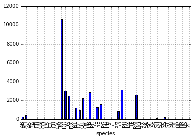 Weight by species plot
We can also look at how many animals were captured in each plot:
total_count=surveys_df.record_id.groupby(surveys_df['plot']).nunique()
# let's plot that too
total_count.plot(kind='bar');
Challenge Activities
- Create a plot of average weight across all species per plot.
- Create a plot of total males versus total females for the entire dataset.
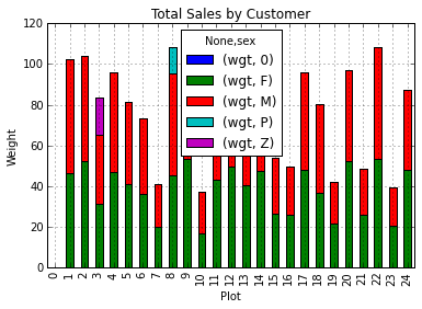
Summary Plotting Challenge
Create a stacked bar plot, with weight on the Y axis, and the stacked variables being sex. The plot should show total weight by sex for each plot. Some tips are below to help you solve this challenge:
- For more on Pandas plots, visit this link.
- You can use the code that follows to create a stacked bar plot but the data need to be in individual columns like this where each value is a mean weight. The first column represents the plot number and the second and third columns represent the sex, like this:
            wgt
sex             F               M
plot
1       46.311138   55.950560
2       52.561845   51.391382

my_plot=data.plot(kind='bar',stacked=True,title="Total Weight by Plot and Sex")
my_plot.set_xlabel("Plot")
my_plot.set_ylabel("Weight")
- You can use the
.unstack()method to transform grouped data into columns for each plotting. Try running `surveys_df.unstack' and see what it yields.